36. Cass-Koopmans Model with Distorting Taxes#
36.1. Overview#
This lecture studies effects of foreseen fiscal and technology shocks on competitive equilibrium prices and quantities in a nonstochastic version of a Cass-Koopmans growth model with features described in this QuantEcon lecture Cass-Koopmans Competitive Equilibrium.
This model is discussed in more detail in chapter 11 of [Ljungqvist and Sargent, 2018].
We use the model as a laboratory to experiment with numerical techniques for approximating equilibria and to display the structure of dynamic models in which decision makers have perfect foresight about future government decisions.
Following a classic paper by Robert E. Hall [Hall, 1971], we augment a nonstochastic version of the Cass-Koopmans optimal growth model with a government that purchases a stream of goods and that finances its purchases with an sequences of several distorting flat-rate taxes.
Distorting taxes prevent a competitive equilibrium allocation from solving a planning problem.
Therefore, to compute an equilibrium allocation and price system, we solve a system of nonlinear difference equations consisting of the first-order conditions for decision makers and the other equilibrium conditions.
We present two ways to approximate an equilibrium:
The first is a shooting algorithm like the one that we deployed in Cass-Koopmans Competitive Equilibrium.
The second method is a root-finding algorithm that minimizes residuals from the first-order conditions of the consumer and representative firm.
After studying the behavior of the closed one-country model, we study a two-country version of the model that is closely related to Mendoza and Tesar [1998].
36.2. The Economy#
36.2.1. Technology#
Feasible allocations satisfy
where
Physical capital evolves according to
where
It is sometimes convenient to eliminate
36.2.2. Components of a competitive equilibrium#
All trades occurring at time
The representative household owns capital, makes investment decisions, and rents capital and labor to a representative production firm.
The representative firm uses capital and labor to produce goods with the production function
A price system is a triple of sequences
The prices
The presence of a government distinguishes this lecture from Cass-Koopmans Competitive Equilibrium.
Government purchases of goods at time
A government expenditure plan is a sequence
A government tax plan is a
Because lump-sum taxes
Nevertheless, we include all of these taxes because, like [Hall, 1971], they allow us to analyze how various taxes distort production and consumption decisions.
In the experiment section, we shall see how variations in government tax plan affect the transition path and equilibrium.
36.2.3. Representative Household#
A representative household has preferences over nonnegative streams of a single consumption good
where
The representative hßousehold maximizes (36.2) subject to the single budget constraint:
Here we have assumed that the government gives a depreciation allowance
36.2.4. Government#
Government plans
Given a budget-feasible government policy
36.3. Equilibrium#
Definition 36.1
A competitive equilibrium with distorting taxes is a budget-feasible government policy, a feasible allocation, and a price system for which, given the price system and the government policy, the allocation solves the household’s problem and the firm’s problem.
36.4. No-arbitrage Condition#
A no-arbitrage argument implies a restriction on prices and tax rates across time.
By rearranging (36.3) and group
The household inherits a given
The household’s budget constraint (36.3) must be bounded in equilibrium due to finite resources.
This imposes a restriction on price and tax sequences.
Specifically, for
If they were strictly positive (negative), the household could arbitrarily increase (decrease) the right-hand side of (36.3) by selecting an arbitrarily large positive (negative)
For strictly positive terms, the household could purchase large capital stocks
For strictly negative terms, the household could engage in “short selling” synthetic units of capital. Both cases would make (36.3) unbounded.
Hence, by setting the terms multiplying
Moreover, we have terminal condition:
Zero-profit conditions for the representative firm impose additional restrictions on equilibrium prices and quantities.
The present value of the firm’s profits is
Applying Euler’s theorem on linearly homogeneous functions to
No-arbitrage (or zero-profit) conditions are:
36.5. Household’s First Order Condition#
Household maximize (36.2) under (36.3).
Let
First-order necessary conditions for the representative household’s problem are
and
Rearranging (36.10) and (36.11), we have
Plugging (36.12) into (36.8) and replacing
36.6. Computing Equilibria#
To compute an equilibrium, we seek a price system
36.7. Python Code#
We require the following imports
import numpy as np
from scipy.optimize import root
import matplotlib.pyplot as plt
from collections import namedtuple
from mpmath import mp, mpf
from warnings import warn

# Set the precision
mp.dps = 40
mp.pretty = True
We use the mpmath library to perform high-precision arithmetic in the shooting algorithm in cases where the solution diverges due to numerical instability.
Note
In the functions below, we include routines to handle the growth component, which will be discussed further in the section Exogenous growth.
We include them here to avoid code duplication.
We set the following parameters
# Create a namedtuple to store the model parameters
Model = namedtuple("Model",
            ["β", "γ", "δ", "α", "A"])

def create_model(β=0.95, # discount factor
                 γ=2.0,  # relative risk aversion coefficient
                 δ=0.2,  # depreciation rate
                 α=0.33, # capital share
                 A=1.0   # TFP
                 ):
    """Create a model instance."""
    return Model(β=β, γ=γ, δ=δ, α=α, A=A)

model = create_model()

# Total number of periods
S = 100
36.7.1. Inelastic Labor Supply#
In this lecture, we consider the special case where
We rewrite (36.1) with
def next_k(k_t, g_t, c_t, model, μ_t=1):
    """
    Capital next period: k_{t+1} = f(k_t) + (1 - δ) * k_t - c_t - g_t
    with optional growth adjustment: k_{t+1} = (f(k_t) + (1 - δ) * k_t - c_t - g_t) / μ_{t+1}
    """
    return (f(k_t, model) + (1 - model.δ) * k_t - g_t - c_t) / μ_t
By the properties of a linearly homogeneous production function, we have
Substituting (36.12), (36.9), and (36.15) into (36.7), we obtain the Euler equation
This can be simplified to:
Equation (36.17) will appear prominently in our equilibrium computation algorithms.
36.7.2. Steady state#
Tax rates and government expenditures act as forcing functions for difference equations (36.15) and (36.17).
Define
Represent the second-order difference equation as:
We assume that a government policy reaches a steady state such that
The terminal steady-state capital stock
From difference equation (36.17), we can infer a restriction on the steady-state:
36.7.3. Other equilibrium quantities and prices#
Price:
def compute_q_path(c_path, model, S=100, A_path=None):
    """
    Compute q path: q_t = (β^t * u'(c_t)) / u'(c_0)
    with optional A_path for growth models.
    """
    A = np.ones_like(c_path) if A_path is None else np.asarray(A_path)
    q_path = np.zeros_like(c_path)
    for t in range(S):
        q_path[t] = (model.β ** t *
                         u_prime(c_path[t], model, A[t])) / u_prime(c_path[0], model, A[0])
    return q_path
Capital rental rate
def compute_η_path(k_path, model, S=100, A_path=None):
    """
    Compute η path: η_t = f'(k_t)
    with optional A_path for growth models.
    """
    A = np.ones_like(k_path) if A_path is None else np.asarray(A_path)
    η_path = np.zeros_like(k_path)
    for t in range(S):
        η_path[t] = f_prime(k_path[t], model, A[t])
    return η_path
Labor rental rate:
def compute_w_path(k_path, η_path, model, S=100, A_path=None):
    """
    Compute w path: w_t = f(k_t) - k_t * f'(k_t)
    with optional A_path for growth models.
    """
    A = np.ones_like(k_path) if A_path is None else np.asarray(A_path)
    w_path = np.zeros_like(k_path)
    for t in range(S):
        w_path[t] = f(k_path[t], model, A[t]) - k_path[t] * η_path[t]
    return w_path
Gross one-period return on capital:
def compute_R_bar(τ_ct, τ_ctp1, τ_ktp1, k_tp1, model):
    """
    Gross one-period return on capital:
    R_bar = [(1 + τ_c_t) / (1 + τ_c_{t+1})]
        * { [1 - τ_k_{t+1}] * [f'(k_{t+1}) - δ] + 1 }
    """
    return ((1 + τ_ct) / (1 + τ_ctp1)) * (
        (1 - τ_ktp1) * (f_prime(k_tp1, model) - model.δ) + 1)
def compute_R_bar_path(shocks, k_path, model, S=100):
    """
    Compute R_bar path over time.
    """
    R_bar_path = np.zeros(S + 1)
    for t in range(S):
        R_bar_path[t] = compute_R_bar(
            shocks['τ_c'][t], shocks['τ_c'][t + 1], shocks['τ_k'][t + 1],
            k_path[t + 1], model)
    R_bar_path[S] = R_bar_path[S - 1]
    return R_bar_path
One-period discount factor:
Net one-period rate of interest:
By (36.22) and
Then by (36.23), we have
Rearranging the above equation, we have
def compute_rts_path(q_path, S, t):
    """
    Compute r path:
    r_t,t+s = - (1/s) * ln(q_{t+s} / q_t)
    """
    s = np.arange(1, S + 1)
    q_path = np.array([float(q) for q in q_path])

    with np.errstate(divide='ignore', invalid='ignore'):
        rts_path = - np.log(q_path[t + s] / q_path[t]) / s
    return rts_path
36.8. Some functional forms#
We assume that the representative household’ period utility has the following CRRA (constant relative risk aversion) form
def u_prime(c, model, A_t=1):
    """
    Marginal utility: u'(c) = c^{-γ}
    with optional technology adjustment: u'(cA) = (cA)^{-γ}
    """
    return (c * A_t) ** (-model.γ)
By substituting (36.21) into (36.17), we obtain
def next_c(c_t, R_bar, model, μ_t=1):
    """
    Consumption next period: c_{t+1} = c_t * (β * R̄)^{1/γ}
    with optional growth adjustment: c_{t+1} = c_t * (β * R_bar)^{1/γ} * μ_{t+1}^{-1}
    """
    return c_t * (model.β * R_bar) ** (1 / model.γ) / μ_t
For the production function we assume a Cobb-Douglas form:
def f(k, model, A=1):
    """
    Production function: f(k) = A * k^{α}
    """
    return A * k ** model.α

def f_prime(k, model, A=1):
    """
    Marginal product of capital: f'(k) = α * A * k^{α - 1}
    """
    return model.α * A * k ** (model.α - 1)
36.9. Computation#
We describe two ways to compute an equilibrium:
a shooting algorithm
a residual-minimization method that focuses on imposing Euler equation (36.17) and the feasibility condition (36.15).
36.9.1. Shooting Algorithm#
This algorithm deploys the following steps.
Solve the equation (36.19) for the terminal steady-state capital
Select a large time index
Use the equation (36.24) to determine
Iterate step 3 to compute candidate values
Compute the difference
Adjust
The following code implements these steps.
# Steady-state calculation
def steady_states(model, g_ss, τ_k_ss=0.0, μ_ss=None):
    """
    Calculate steady state values for capital and
    consumption with optional A_path for growth models.
    """

    β, δ, α, γ = model.β, model.δ, model.α, model.γ

    A = model.A or 1.0

    # growth‐adjustment in the numerator: μ^γ or 1
    μ_eff = μ_ss**γ if μ_ss is not None else 1.0

    num = δ + (μ_eff/β - 1) / (1 - τ_k_ss)
    k_ss = (num / (α * A)) ** (1 / (α - 1))

    c_ss = (
        A * k_ss**α - δ * k_ss - g_ss
        if μ_ss is None
        else k_ss**α + (1 - δ - μ_ss) * k_ss - g_ss
    )

    return k_ss, c_ss

def shooting_algorithm(
    c0, k0, shocks, S, model, A_path=None):
    """
    Shooting algorithm for given initial c0 and k0
    with optional A_path for growth models.
    """
    # unpack & mpf‐ify shocks, fill μ with ones if missing
    g = np.array(list(map(mpf, shocks['g'])), dtype=object)
    τ_c = np.array(list(map(mpf, shocks['τ_c'])), dtype=object)
    τ_k = np.array(list(map(mpf, shocks['τ_k'])), dtype=object)
    μ = (np.array(list(map(mpf, shocks['μ'])), dtype=object)
              if 'μ' in shocks else np.ones_like(g))
    A = np.ones_like(g) if A_path is None else A_path

    k_path = np.empty(S+1, dtype=object)
    c_path = np.empty(S+1, dtype=object)
    k_path[0], c_path[0] = mpf(k0), mpf(c0)

    for t in range(S):
        k_t, c_t = k_path[t], c_path[t]
        k_tp1 = next_k(k_t, g[t], c_t, model, μ[t+1])
        if k_tp1 < 0:
            return None, None
        k_path[t+1] = k_tp1

        R_bar = compute_R_bar(
            τ_c[t], τ_c[t+1], τ_k[t+1], k_tp1, model
        )
        c_tp1 = next_c(c_t, R_bar, model, μ[t+1])
        if c_tp1 < 0:
            return None, None
        c_path[t+1] = c_tp1

    return k_path, c_path


def bisection_c0(
    c0_guess, k0, shocks, S, model, tol=mpf('1e-6'),
    max_iter=1000, verbose=False, A_path=None):
    """
    Bisection method to find initial c0
    """
    # steady‐state uses last shocks (μ=1 if missing)
    g_last    = mpf(shocks['g'][-1])
    τ_k_last  = mpf(shocks['τ_k'][-1])
    μ_last    = mpf(shocks['μ'][-1]) if 'μ' in shocks else mpf('1')
    k_ss_fin, _ = steady_states(model, g_last, τ_k_last, μ_last)

    c0_lo, c0_hi = mpf('0'), f(k_ss_fin, model)
    c0 = mpf(c0_guess)

    for i in range(1, max_iter+1):
        k_path, _ = shooting_algorithm(c0, k0, shocks, S, model, A_path)
        if k_path is None:
            if verbose:
                print(f"[{i}] shoot failed at c0={c0}")
            c0_hi = c0
        else:
            err = k_path[-1] - k_ss_fin
            if verbose and i % 100 == 0:
                print(f"[{i}] c0={c0}, err={err}")
            if abs(err) < tol:
                if verbose:
                    print(f"Converged after {i} iter")
                return c0
            # update bounds in one line
            c0_lo, c0_hi = (c0, c0_hi) if err > 0 else (c0_lo, c0)
        c0 = (c0_lo + c0_hi) / mpf('2')

    warn(f"bisection did not converge after {max_iter} iters; returning c0={c0}")
    return c0


def run_shooting(
    shocks, S, model, A_path=None,
    c0_finder=bisection_c0, shooter=shooting_algorithm):
    """
    Compute initial SS, find c0, and return [k,c] paths
    with optional A_path for growth models.
    """
    # initial SS at t=0 (μ=1 if missing)
    g0    = mpf(shocks['g'][0])
    τ_k0  = mpf(shocks['τ_k'][0])
    μ0    = mpf(shocks['μ'][0]) if 'μ' in shocks else mpf('1')
    k0, c0 = steady_states(model, g0, τ_k0, μ0)

    optimal_c0 = c0_finder(c0, k0, shocks, S, model, A_path=A_path)
    print(f"Model: {model}\nOptimal initial consumption c0 = {mpf(optimal_c0)}")

    k_path, c_path = shooter(optimal_c0, k0, shocks, S, model, A_path)
    return np.column_stack([k_path, c_path])
36.9.2. Experiments#
Let’s run some experiments.
A foreseen once-and-for-all increase in
A foreseen once-and-for-all increase in
A foreseen once-and-for-all increase in
A foreseen one-time increase in
To start, we prepare sequences that we’ll used to initialize our iterative algorithm.
We will start from an initial steady state and apply shocks at an the indicated time.
def plot_results(
    solution, k_ss, c_ss, shocks, shock_param, axes, model,
    A_path=None, label='', linestyle='-', T=40):
    """
    Plot simulation results (k, c, R, η, and a policy shock)
    with optional A_path for growth models.
    """
    k_path = solution[:, 0]
    c_path = solution[:, 1]
    T = min(T, k_path.size)

    # handle growth parameters
    μ0 = shocks['μ'][0] if 'μ' in shocks else 1.0
    A0 = A_path[0] if A_path is not None else (model.A or 1.0)

    # steady‐state lines
    R_bar_ss = (1 / model.β) * (μ0**model.γ)
    η_ss     = model.α * A0 * k_ss**(model.α - 1)

    # plot k
    axes[0].plot(k_path[:T], linestyle=linestyle, label=label)
    axes[0].axhline(k_ss, linestyle='--', color='black')
    axes[0].set_title('k')

    # plot c
    axes[1].plot(c_path[:T], linestyle=linestyle, label=label)
    axes[1].axhline(c_ss, linestyle='--', color='black')
    axes[1].set_title('c')

    # plot R bar
    S_full    = k_path.size - 1
    R_bar_path = compute_R_bar_path(shocks, k_path, model, S_full)
    axes[2].plot(R_bar_path[:T], linestyle=linestyle, label=label)
    axes[2].axhline(R_bar_ss, linestyle='--', color='black')
    axes[2].set_title(r'$\bar{R}$')

    # plot η
    η_path = compute_η_path(k_path, model, S_full)
    axes[3].plot(η_path[:T], linestyle=linestyle, label=label)
    axes[3].axhline(η_ss, linestyle='--', color='black')
    axes[3].set_title(r'$\eta$')

    # plot shock
    shock_series = np.array(shocks[shock_param], dtype=object)
    axes[4].plot(shock_series[:T], linestyle=linestyle, label=label)
    axes[4].axhline(shock_series[0], linestyle='--', color='black')
    axes[4].set_title(rf'${shock_param}$')

    if label:
        for ax in axes[:5]:
            ax.legend()
Experiment 1: Foreseen once-and-for-all increase in
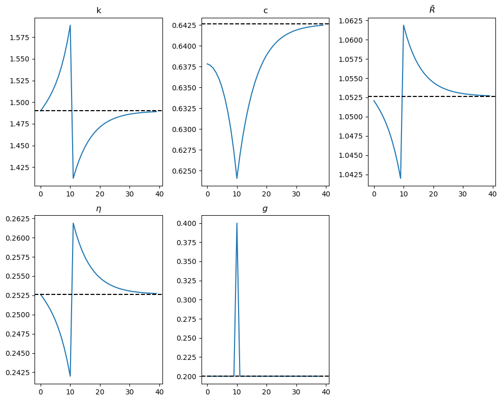
The figure below shows consequences of a foreseen permanent increase in
# Define shocks as a dictionary
shocks = {
    'g': np.concatenate(
        (np.repeat(0.2, 10), np.repeat(0.4, S - 9))
    ),
    'τ_c': np.repeat(0.0, S + 1),
    'τ_k': np.repeat(0.0, S + 1)
}

k_ss_initial, c_ss_initial = steady_states(model,
                                           shocks['g'][0],
                                           shocks['τ_k'][0])

print(f"Steady-state capital: {k_ss_initial:.4f}")
print(f"Steady-state consumption: {c_ss_initial:.4f}")

solution = run_shooting(shocks, S, model)

fig, axes = plt.subplots(2, 3, figsize=(10, 8))
axes = axes.flatten()

plot_results(solution, k_ss_initial,
             c_ss_initial, shocks, 'g', axes, model, T=40)

for ax in axes[5:]:
    fig.delaxes(ax)

plt.tight_layout()
plt.show()
Steady-state capital: 1.4900
Steady-state consumption: 0.6426
Model: Model(β=0.95, γ=2.0, δ=0.2, α=0.33, A=1.0)
Optimal initial consumption c0 = 0.6092419528879239645312185699727132533517
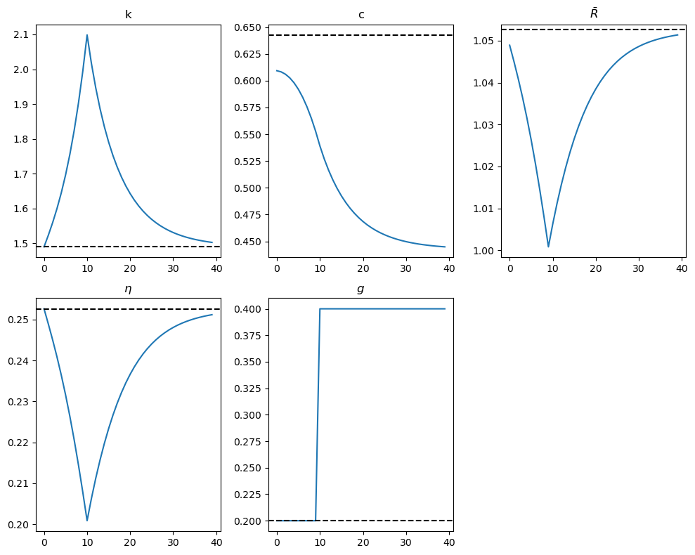
The above figures indicate that an equilibrium consumption smoothing mechanism is at work, driven by the representative consumer’s preference for smooth consumption paths coming from the curvature of its one-period utility function.
The steady-state value of the capital stock remains unaffected:
This follows from the fact that
Consumption begins to decline gradually before time
Households reduce consumption to offset government spending, which is financed through increased lump-sum taxes.
The competitive economy signals households to consume less through an increase in the stream of lump-sum taxes.
Households, caring about the present value rather than the timing of taxes, experience an adverse wealth effect on consumption, leading to an immediate response.
Capital gradually accumulates between time
This temporal variation in capital stock smooths consumption over time, driven by the representative consumer’s consumption-smoothing motive.
Let’s collect the procedures used above into a function that runs the solver and draws plots for a given experiment
Show code cell source
def experiment_model(
    shocks, S, model, A_path=None, solver=run_shooting,
    plot_func=plot_results, policy_shock='g', T=40):
    """
    Run the shooting algorithm and plot results.
    """
    # initial steady state (μ0=None if no growth)
    g0   = mpf(shocks['g'][0])
    τk0  = mpf(shocks['τ_k'][0])
    μ0   = mpf(shocks['μ'][0]) if 'μ' in shocks else None
    k_ss, c_ss = steady_states(model, g0, τk0, μ0)

    print(f"Steady-state capital: {float(k_ss):.4f}")
    print(f"Steady-state consumption: {float(c_ss):.4f}")
    print('-'*64)

    fig, axes = plt.subplots(2, 3, figsize=(10, 8))
    axes = axes.flatten()

    sol = solver(shocks, S, model, A_path)
    plot_func(
        sol, k_ss, c_ss, shocks, policy_shock, axes, model,
        A_path=A_path, T=T
    )

    # remove unused axes
    for ax in axes[5:]:
        fig.delaxes(ax)

    plt.tight_layout()
    plt.show()
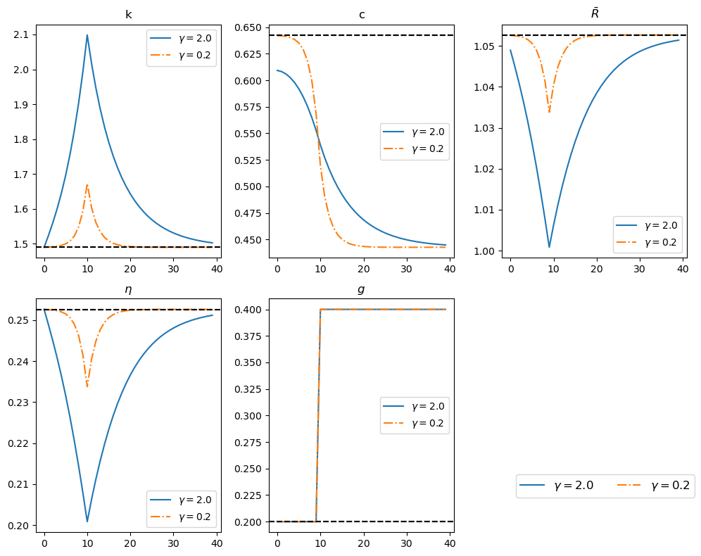
The following figure compares responses to a foreseen increase in
our original economy with
an otherwise identical economy with
This comparison interest us because the utility curvature parameter
# Solve the model using shooting
solution = run_shooting(shocks, S, model)

# Compute the initial steady states
k_ss_initial, c_ss_initial = steady_states(model,
                                           shocks['g'][0],
                                           shocks['τ_k'][0])

# Plot the solution for γ=2
fig, axes = plt.subplots(2, 3, figsize=(10, 8))
axes = axes.flatten()

label = fr"$\gamma = {model.γ}$"
plot_results(solution, k_ss_initial, c_ss_initial,
             shocks, 'g', axes, model, label=label,
             T=40)

# Solve and plot the result for γ=0.2
model_γ2 = create_model(γ=0.2)
solution = run_shooting(shocks, S, model_γ2)

plot_results(solution, k_ss_initial, c_ss_initial,
             shocks, 'g', axes, model_γ2,
             label=fr"$\gamma = {model_γ2.γ}$",
             linestyle='-.', T=40)

handles, labels = axes[0].get_legend_handles_labels()
fig.legend(handles, labels, loc='lower right',
           ncol=3, fontsize=14, bbox_to_anchor=(1, 0.1))

for ax in axes[5:]:
    fig.delaxes(ax)

plt.tight_layout()
plt.show()
Model: Model(β=0.95, γ=2.0, δ=0.2, α=0.33, A=1.0)
Optimal initial consumption c0 = 0.6092419528879239645312185699727132533517
Model: Model(β=0.95, γ=0.2, δ=0.2, α=0.33, A=1.0)
Optimal initial consumption c0 = 0.6420330412987902926414768724607623681745
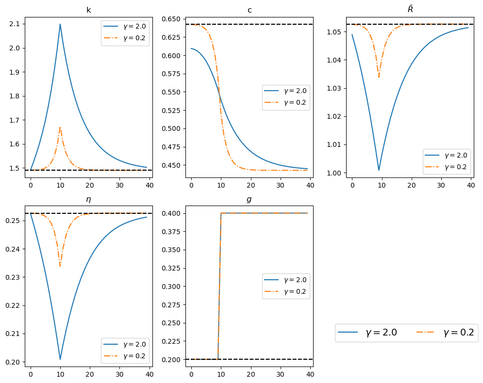
The outcomes indicate that lowering
Consumption path:
When
For
Capital stock path:
With
There are also smaller fluctuations in
Let’s write another function that runs the solver and draws plots for these two experiments
Show code cell source
def experiment_two_models(
    shocks, S, model_1, model_2, solver=run_shooting, plot_func=plot_results,
    policy_shock='g', legend_label_fun=None, T=40, A_path=None):
    """
    Compare and plot the shooting algorithm paths for two models.
    """
    is_growth = 'μ' in shocks
    μ0 = mpf(shocks['μ'][0]) if is_growth else None

    # initial steady states for both models
    g0   = mpf(shocks['g'][0])
    τk0  = mpf(shocks['τ_k'][0])
    k_ss1, c_ss1 = steady_states(model_1, g0, τk0, μ0)
    k_ss2, c_ss2 = steady_states(model_2, g0, τk0, μ0)

    # print both
    print(f"Model 1 (γ={model_1.γ}): steady state k={float(k_ss1):.4f}, c={float(c_ss1):.4f}")
    print(f"Model 2 (γ={model_2.γ}): steady state k={float(k_ss2):.4f}, c={float(c_ss2):.4f}")
    print('-'*64)

    # default legend labels
    if legend_label_fun is None:
        legend_label_fun = lambda m: fr"$\gamma = {m.γ}$"

    # prepare figure
    fig, axes = plt.subplots(2, 3, figsize=(10, 8))
    axes = axes.flatten()

    # loop over (model, steady‐state, linestyle)
    for model, (k_ss, c_ss), ls in [
        (model_1, (k_ss1, c_ss1), '-'),
        (model_2, (k_ss2, c_ss2), '-.')
    ]:
        sol = solver(shocks, S, model, A_path)
        plot_func(sol, k_ss, c_ss, shocks, policy_shock, axes,
                  model, A_path=A_path,
                  label=legend_label_fun(model),
                  linestyle=ls, T=T)

    # shared legend in lower‐right
    handles, labels = axes[0].get_legend_handles_labels()
    fig.legend(
        handles, labels, loc='lower right', ncol=2,
        fontsize=12, bbox_to_anchor=(1, 0.1))

    # drop the unused subplot
    for ax in axes[5:]:
        fig.delaxes(ax)

    plt.tight_layout()
    plt.show()
Now we plot other equilibrium quantities:
def plot_prices(solution, c_ss, shock_param, axes,
                model, label='', linestyle='-', T=40):
    """
    Compares and plots prices
    """
    α, β, δ, γ, A = model.α, model.β, model.δ, model.γ, model.A

    k_path = solution[:, 0]
    c_path = solution[:, 1]

    # Plot for c
    axes[0].plot(c_path[:T], linestyle=linestyle, label=label)
    axes[0].axhline(c_ss, linestyle='--', color='black')
    axes[0].set_title('c')

    # Plot for q
    q_path = compute_q_path(c_path, model, S=S)
    axes[1].plot(q_path[:T], linestyle=linestyle, label=label)
    axes[1].plot(β**np.arange(T), linestyle='--', color='black')
    axes[1].set_title('q')

    # Plot for r_{t,t+1}
    R_bar_path = compute_R_bar_path(shocks, k_path, model, S)
    axes[2].plot(R_bar_path[:T] - 1, linestyle=linestyle, label=label)
    axes[2].axhline(1 / β - 1, linestyle='--', color='black')
    axes[2].set_title('$r_{t,t+1}$')

    # Plot for r_{t,t+s}
    for style, s in zip(['-', '-.', '--'], [0, 10, 60]):
        rts_path = compute_rts_path(q_path, T, s)
        axes[3].plot(rts_path, linestyle=style,
                     color='black' if style == '--' else None,
                     label=f'$t={s}$')
        axes[3].set_xlabel('s')
        axes[3].set_title('$r_{t,t+s}$')

    # Plot for g
    axes[4].plot(shocks[shock_param][:T], linestyle=linestyle, label=label)
    axes[4].axhline(shocks[shock_param][0], linestyle='--', color='black')
    axes[4].set_title(shock_param)
For
solution = run_shooting(shocks, S, model)

fig, axes = plt.subplots(2, 3, figsize=(10, 8))
axes = axes.flatten()

plot_prices(solution, c_ss_initial, 'g', axes, model, T=40)

for ax in axes[5:]:
    fig.delaxes(ax)

handles, labels = axes[3].get_legend_handles_labels()
fig.legend(handles, labels, title=r"$r_{t,t+s}$ with ", loc='lower right',
           ncol=3, fontsize=10, bbox_to_anchor=(1, 0.1))
plt.tight_layout()
plt.show()
Model: Model(β=0.95, γ=2.0, δ=0.2, α=0.33, A=1.0)
Optimal initial consumption c0 = 0.6092419528879239645312185699727132533517

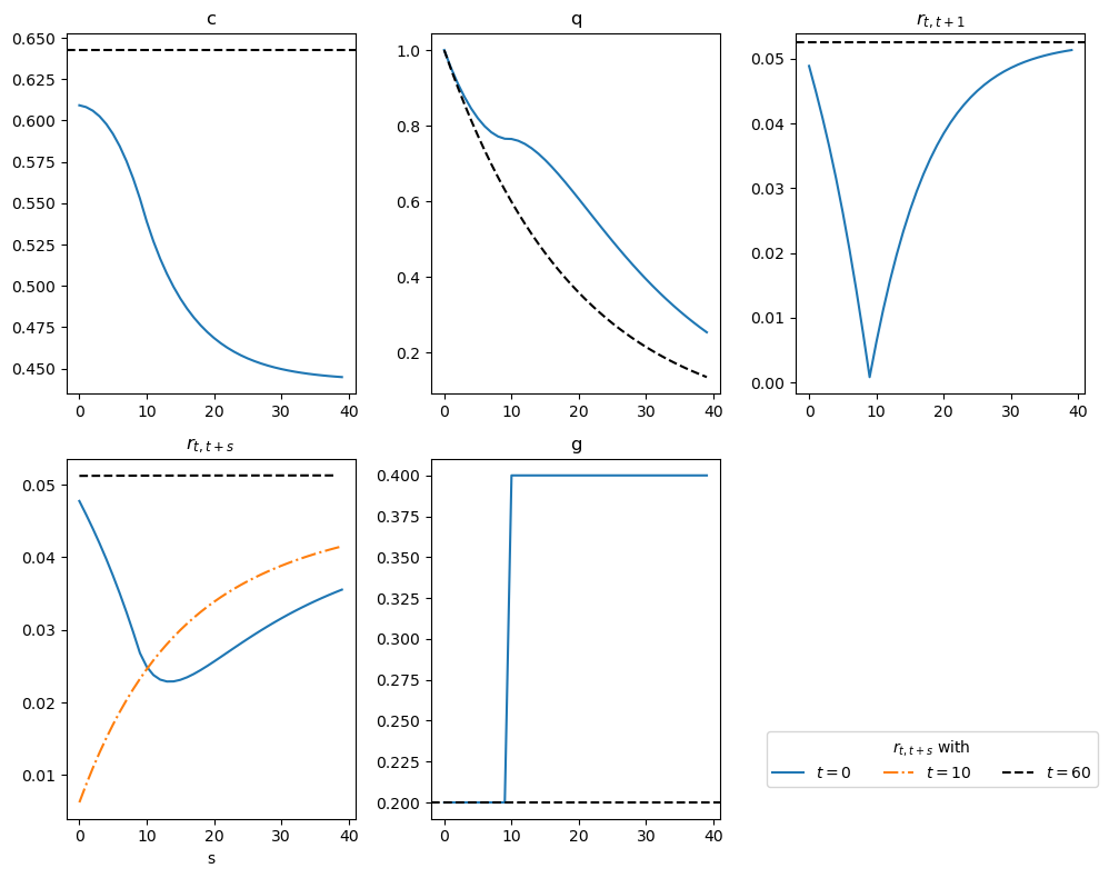
The second panel on the top compares
The fourth panel shows the term structure of interest rates at
Notice that, by
At
This upward slope reflects the expected increase in the rate of growth of consumption over time, as shown in the consumption panel.
At
It declines until maturity at
After
This pattern aligns with the pattern of consumption growth in the first two figures,
which declines at an increasing rate until
Experiment 2: Foreseen once-and-for-all increase in
With an inelastic labor supply, the Euler equation (36.16) and the other equilibrium conditions show that
constant consumption taxes do not distort decisions, but
anticipated changes in them do.
Indeed, (36.16) or (36.17) indicates that a foreseen in-
crease in
The following figure portrays the response to a foreseen increase in the consumption tax
shocks = {
    'g': np.repeat(0.2, S + 1),
    'τ_c': np.concatenate((np.repeat(0.0, 10), np.repeat(0.2, S - 9))),
    'τ_k': np.repeat(0.0, S + 1)
}

experiment_model(shocks, S, model,
                 solver=run_shooting,
                 plot_func=plot_results,
                 policy_shock='τ_c')
Steady-state capital: 1.4900
Steady-state consumption: 0.6426
----------------------------------------------------------------
Model: Model(β=0.95, γ=2.0, δ=0.2, α=0.33, A=1.0)
Optimal initial consumption c0 = 0.6492795614681543372301864705195788398396
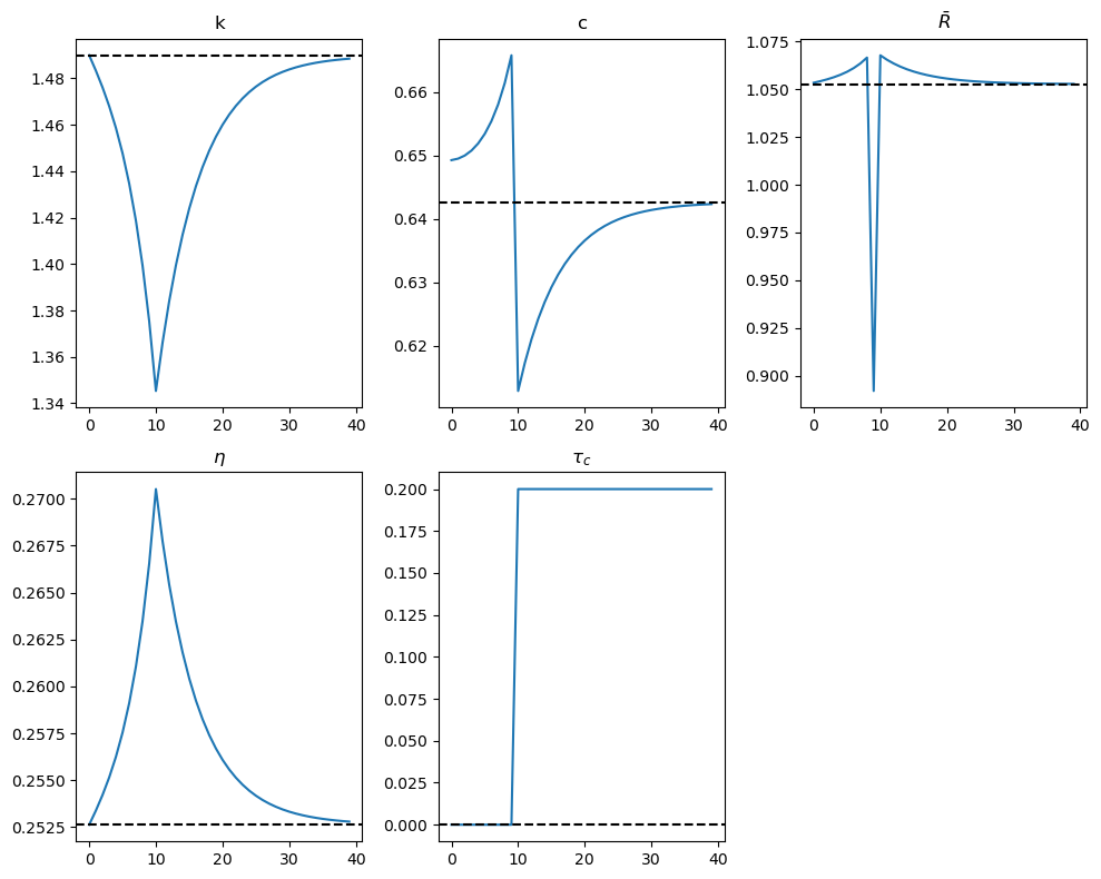
Evidently all variables in the figures above eventually return to their initial steady-state values.
The anticipated increase in
At
Anticipation of the increase in
This is followed by a consumption binge that sends the capital stock downward until
Between
The decline in the capital stock raises
The equilibrium conditions require the growth rate of consumption to rise until
At
The jump in
After
The effects of anticipated distortion are over, and the economy gradually adjusts to the lower capital stock.
Capital must now rise, requiring austerity —consumption plummets after
The interest rate gradually declines, and consumption grows at a diminishing rate along the path to the terminal steady-state.
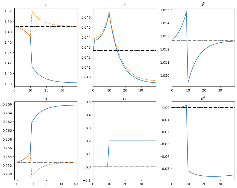
Experiment 3: Foreseen once-and-for-all increase in
For the two
shocks = {
    'g': np.repeat(0.2, S + 1),
    'τ_c': np.repeat(0.0, S + 1),
    'τ_k': np.concatenate((np.repeat(0.0, 10), np.repeat(0.2, S - 9)))
}

experiment_two_models(shocks, S, model, model_γ2,
                solver=run_shooting,
                 plot_func=plot_results,
                 policy_shock='τ_k')
Model 1 (γ=2.0): steady state k=1.4900, c=0.6426
Model 2 (γ=0.2): steady state k=1.4900, c=0.6426
----------------------------------------------------------------
Model: Model(β=0.95, γ=2.0, δ=0.2, α=0.33, A=1.0)
Optimal initial consumption c0 = 0.6448856400318608460996300822707014890199
Model: Model(β=0.95, γ=0.2, δ=0.2, α=0.33, A=1.0)
Optimal initial consumption c0 = 0.6428407772240506727464152695921513767415
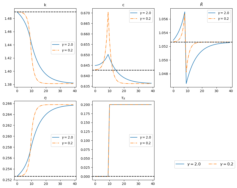
The path of government expenditures remains fixed
the increase in
The figure shows that:
Anticipation of the increase in
Variations in
Transition dynamics push
Consumption is lower due to reduced output from the lower capital stock.
Smoother consumption paths occur when
So far we have explored consequences of foreseen once-and-for-all changes in government policy. Next we describe some experiments in which there is a foreseen one-time change in a policy variable (a “pulse”).
Experiment 4: Foreseen one-time increase in
g_path = np.repeat(0.2, S + 1)
g_path[10] = 0.4

shocks = {
    'g': g_path,
    'τ_c': np.repeat(0.0, S + 1),
    'τ_k': np.repeat(0.0, S + 1)
}

experiment_model(shocks, S, model,
                 solver=run_shooting,
                 plot_func=plot_results,
                 policy_shock='g')
Steady-state capital: 1.4900
Steady-state consumption: 0.6426
----------------------------------------------------------------
Model: Model(β=0.95, γ=2.0, δ=0.2, α=0.33, A=1.0)
Optimal initial consumption c0 = 0.6378298012463969247674771825320030214755
The figure indicates how:
Consumption:
Drops immediately upon announcement of the policy and continues to decline over time in anticipation of the one-time surge in
After the shock at
Capital and
Before
At
36.9.3. Method 2: Residual Minimization#
The second method involves minimizing residuals (i.e., deviations from equalities) of the following equations:
# Euler's equation and feasibility condition
def euler_residual(c_t, c_tp1, τ_c_t, τ_c_tp1, τ_k_tp1, k_tp1, model, μ_tp1=1):
    """
    Computes the residuals for Euler's equation
    with optional growth model parameters μ_tp1.
    """
    R_bar = compute_R_bar(τ_c_t, τ_c_tp1, τ_k_tp1, k_tp1, model)

    c_expected = next_c(c_t, R_bar, model, μ_tp1)

    return c_expected / c_tp1 - 1.0

def feasi_residual(k_t, k_tm1, c_tm1, g_t, model, μ_t=1):
    """
    Computes the residuals for feasibility condition
    with optional growth model parameter μ_t.
    """
    k_t_expected = next_k(k_tm1, g_t, c_tm1, model, μ_t)
    return k_t_expected - k_t
The algorithm proceeds follows:
Find initial steady state
Initialize a sequence of initial guesses
Compute residuals
Compute the Euler equation residual for
Compute the feasibility condition residual for
Compute the residual for the initial condition for
Compute the residual for the terminal condition for
Iteratively adjust guesses for
def compute_residuals(vars_flat, k_init, S, shock_paths, model):
    """
    Compute the residuals for the Euler equation and feasibility condition.
    """
    g, τ_c, τ_k, μ = (shock_paths[key] for key in ('g','τ_c','τ_k','μ'))
    k, c = vars_flat.reshape((S+1, 2)).T
    res = np.empty(2*S+2, dtype=float)

    # boundary condition on initial capital
    res[0] = k[0] - k_init

    # interior Euler and feasibility
    for t in range(S):
        res[2*t + 1] = euler_residual(
            c[t],    c[t+1],
            τ_c[t],  τ_c[t+1],
            τ_k[t+1],k[t+1],
            model, μ[t+1])
        res[2*t + 2] = feasi_residual(
            k[t+1], k[t], c[t],
            g[t],  model,
            μ[t+1])

    # terminal Euler condition at t=S
    res[-1] = euler_residual(
        c[S],   c[S],
        τ_c[S], τ_c[S],
        τ_k[S], k[S],
        model,
        μ[S])

    return res


def run_min(shocks, S, model, A_path=None):
    """
    Solve for the full (k,c) path by root‐finding the residuals.
    """
    shocks['μ'] = shocks['μ'] if 'μ' in shocks else np.ones_like(shocks['g'])

    # compute the steady‐state to serve as both initial capital and guess
    k_ss, c_ss = steady_states(
        model,
        shocks['g'][0],
        shocks['τ_k'][0],
        shocks['μ'][0]  # =1 if no growth
    )

    # initial guess: flat at the steady‐state
    guess = np.column_stack([
        np.full(S+1, k_ss),
        np.full(S+1, c_ss)
    ]).flatten()

    sol = root(
        compute_residuals,
        guess,
        args=(k_ss, S, shocks, model),
        tol=1e-8
    )

    return sol.x.reshape((S+1, 2))
We found that method 2 did not encounter numerical stability issues, so using mp.mpf is not necessary.
We leave as exercises replicating some of our experiments by using the second method.
Exercise 36.1
Replicate the plots of our four experiments using the second method of residual minimization:
A foreseen once-and-for-all increase in
A foreseen once-and-for-all increase in
A foreseen once-and-for-all increase in
A foreseen one-time increase in
Solution to Exercise 36.1
Here is one solution:
Experiment 1: Foreseen once-and-for-all increase in
shocks = {
    'g': np.concatenate((np.repeat(0.2, 10), np.repeat(0.4, S - 9))),
    'τ_c': np.repeat(0.0, S + 1),
    'τ_k': np.repeat(0.0, S + 1)
}

experiment_model(shocks, S, model, solver=run_min,
                 plot_func=plot_results,
                 policy_shock='g')
Steady-state capital: 1.4900
Steady-state consumption: 0.6426
----------------------------------------------------------------
experiment_two_models(shocks, S, model, model_γ2,
                run_min, plot_results, 'g')
Model 1 (γ=2.0): steady state k=1.4900, c=0.6426
Model 2 (γ=0.2): steady state k=1.4900, c=0.6426
----------------------------------------------------------------
solution = run_min(shocks, S, model)

fig, axes = plt.subplots(2, 3, figsize=(10, 8))
axes = axes.flatten()

plot_prices(solution, c_ss_initial, 'g', axes, model, T=40)

for ax in axes[5:]:
    fig.delaxes(ax)

handles, labels = axes[3].get_legend_handles_labels()
fig.legend(handles, labels, title=r"$r_{t,t+s}$ with ", loc='lower right', ncol=3, fontsize=10, bbox_to_anchor=(1, 0.1))
plt.tight_layout()
plt.show()
Experiment 2: Foreseen once-and-for-all increase in
shocks = {
    'g': np.repeat(0.2, S + 1),
    'τ_c': np.concatenate((np.repeat(0.0, 10), np.repeat(0.2, S - 9))),
    'τ_k': np.repeat(0.0, S + 1)
}

experiment_model(shocks, S, model, solver=run_min,
                 plot_func=plot_results,
                 policy_shock='τ_c')
Steady-state capital: 1.4900
Steady-state consumption: 0.6426
----------------------------------------------------------------
Experiment 3: Foreseen once-and-for-all increase in
shocks = {
    'g': np.repeat(0.2, S + 1),
    'τ_c': np.repeat(0.0, S + 1),
    'τ_k': np.concatenate((np.repeat(0.0, 10), np.repeat(0.2, S - 9)))
}

experiment_two_models(shocks, S, model, model_γ2,
                solver=run_min,
                 plot_func=plot_results,
                 policy_shock='τ_k')
Model 1 (γ=2.0): steady state k=1.4900, c=0.6426
Model 2 (γ=0.2): steady state k=1.4900, c=0.6426
----------------------------------------------------------------
Experiment 4: Foreseen one-time increase in
g_path = np.repeat(0.2, S + 1)
g_path[10] = 0.4

shocks = {
    'g': g_path,
    'τ_c': np.repeat(0.0, S + 1),
    'τ_k': np.repeat(0.0, S + 1)
}

experiment_model(shocks, S, model, solver=run_min,
                 plot_func=plot_results,
                 policy_shock='g')
Steady-state capital: 1.4900
Steady-state consumption: 0.6426
----------------------------------------------------------------
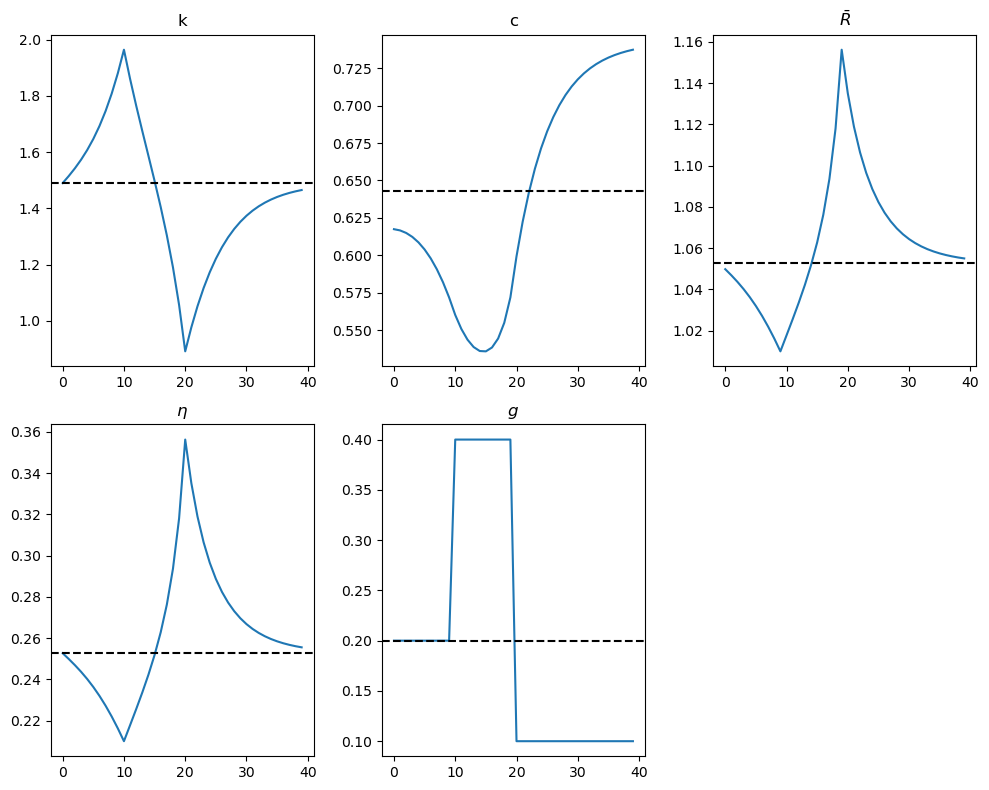
Exercise 36.2
Design a new experiment where the government expenditure
Solution to Exercise 36.2
Here is one solution:
g_path = np.repeat(0.2, S + 1)
g_path[10:20] = 0.4
g_path[20:] = 0.1

shocks = {
    'g': g_path,
    'τ_c': np.repeat(0.0, S + 1),
    'τ_k': np.repeat(0.0, S + 1)
}

experiment_model(shocks, S, model, solver=run_min,
                 plot_func=plot_results,
                 policy_shock='g')
Steady-state capital: 1.4900
Steady-state consumption: 0.6426
----------------------------------------------------------------
36.10. Exogenous growth#
In the previous section, we considered a model without exogenous growth.
We set the term
Now we are ready to consider growth.
To incorporate growth, we modify the production function to be
where
We assume that
and that
# Set the constant A parameter to None
model = create_model(A=None)
def compute_A_path(A0, shocks, S=100):
    """
    Compute A path over time.
    """
    A_path = np.full(S + 1, A0)
    for t in range(1, S + 1):
        A_path[t] = A_path[t-1] * shocks['μ'][t-1]
    return A_path
36.10.1. Inelastic Labor Supply#
By linear homogeneity, the production function can be expressed as
where
We also let
We continue to consider the case of inelastic labor supply.
Based on this, feasibility can be summarized by the following modified version of equation (36.15):
Again, by the properties of a linearly homogeneous production function, we have
Since per capita consumption is now
Thus, substituting (36.21), (36.27) becomes
Assuming that the household’s utility function is the same as before, we have
Thus, the counterpart to (36.24) is
36.10.2. Steady State#
In a steady state,
from which we can compute that the steady-state level of capital per unit of effective labor satisfies
and that
The steady-state level of consumption per unit of effective labor can be found using (36.26):
Since the algorithm and plotting routines are the same as before, we include the steady-state calculations and shooting routine in the section Python Code.
36.10.3. Shooting Algorithm#
Now we can apply the shooting algorithm to compute equilibrium. We augment the vector of shock variables by including
36.10.4. Experiments#
Let’s run some experiments:
A foreseen once-and-for-all increase in
An unforeseen once-and-for-all increase in
36.10.4.1. Experiment 1: A foreseen increase in
The figures below show the effects of a permanent increase in productivity growth
They now measure
shocks = {
    'g': np.repeat(0.2, S + 1),
    'τ_c': np.repeat(0.0, S + 1),
    'τ_k': np.repeat(0.0, S + 1),
    'μ': np.concatenate((np.repeat(1.02, 10), np.repeat(1.025, S - 9)))
}

A_path = compute_A_path(1.0, shocks, S)

k_ss_initial, c_ss_initial = steady_states(model,
                                         shocks['g'][0],
                                         shocks['τ_k'][0],
                                         shocks['μ'][0]
                                        )

print(f"Steady-state capital: {k_ss_initial:.4f}")
print(f"Steady-state consumption: {c_ss_initial:.4f}")

# Run the shooting algorithm with the A_path parameter
solution = run_shooting(shocks, S, model, A_path)

fig, axes = plt.subplots(2, 3, figsize=(10, 8))
axes = axes.flatten()

plot_results(solution, k_ss_initial,
             c_ss_initial, shocks, 'μ', axes, model,
             A_path, T=40)

for ax in axes[5:]:
    fig.delaxes(ax)

plt.tight_layout()
plt.show()
Steady-state capital: 1.1812
Steady-state consumption: 0.5966
Model: Model(β=0.95, γ=2.0, δ=0.2, α=0.33, A=None)
Optimal initial consumption c0 = 0.5971184749344462396270918337183607339919
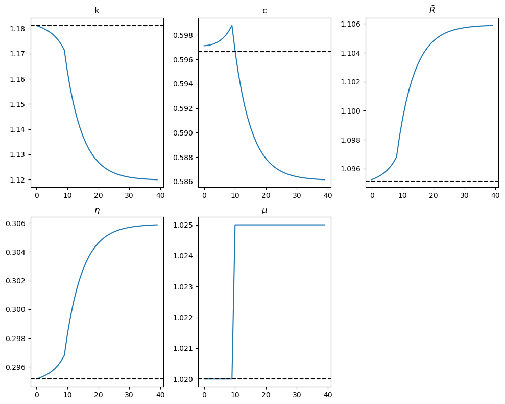
The results in the figures are mainly driven by (36.29)
and imply that a permanent increase in
The figures indicate the following:
As capital becomes more efficient, even with less of it, consumption per capita can be raised.
Consumption smoothing drives an immediate jump in consumption in anticipation of the increase in
The increased productivity of capital leads to an increase in the gross return
Perfect foresight makes the effects of the increase in the growth of capital precede it, with the effect visible at
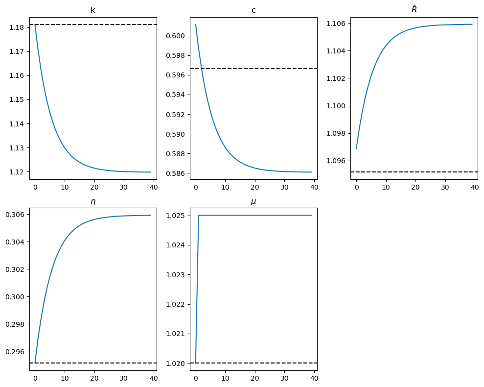
36.10.4.2. Experiment 2: An unforeseen increase in
The figures below show the effects of an immediate jump in
shocks = {
    'g': np.repeat(0.2, S + 1),
    'τ_c': np.repeat(0.0, S + 1),
    'τ_k': np.repeat(0.0, S + 1),
    'μ': np.concatenate((np.repeat(1.02, 1), np.repeat(1.025, S)))
}

A_path = compute_A_path(1.0, shocks, S)

k_ss_initial, c_ss_initial = steady_states(model,
                                           shocks['g'][0],
                                           shocks['τ_k'][0],
                                           shocks['μ'][0]
                                          )

print(f"Steady-state capital: {k_ss_initial:.4f}")
print(f"Steady-state consumption: {c_ss_initial:.4f}")

# Run the shooting algorithm with the A_path parameter
solution = run_shooting(shocks, S, model, A_path)

fig, axes = plt.subplots(2, 3, figsize=(10, 8))
axes = axes.flatten()

plot_results(solution, k_ss_initial,
             c_ss_initial, shocks, 'μ', axes, model, A_path, T=40)

for ax in axes[5:]:
    fig.delaxes(ax)

plt.tight_layout()
plt.show()
Steady-state capital: 1.1812
Steady-state consumption: 0.5966
Model: Model(β=0.95, γ=2.0, δ=0.2, α=0.33, A=None)
Optimal initial consumption c0 = 0.6011494930430641150395883753109588316638
Again, we can collect the procedures used above into a function that runs the solver and draws plots for a given experiment.
def experiment_model(shocks, S, model, A_path, solver, plot_func, policy_shock, T=40):
    """
    Run the shooting algorithm given a model and plot the results.
    """
    k0, c0 = steady_states(model, shocks['g'][0], shocks['τ_k'][0], shocks['μ'][0])

    print(f"Steady-state capital: {k0:.4f}")
    print(f"Steady-state consumption: {c0:.4f}")
    print('-'*64)

    fig, axes = plt.subplots(2, 3, figsize=(10, 8))
    axes = axes.flatten()

    solution = solver(shocks, S, model, A_path)
    plot_func(solution, k0, c0,
              shocks, policy_shock, axes, model, A_path, T=T)

    for ax in axes[5:]:
        fig.delaxes(ax)

    plt.tight_layout()
    plt.show()
shocks = {
    'g': np.repeat(0.2, S + 1),
    'τ_c': np.repeat(0.0, S + 1),
    'τ_k': np.repeat(0.0, S + 1),
    'μ': np.concatenate((np.repeat(1.02, 1), np.repeat(1.025, S)))
}

experiment_model(shocks, S, model, A_path, run_shooting, plot_results, 'μ')
Steady-state capital: 1.1812
Steady-state consumption: 0.5966
----------------------------------------------------------------
Model: Model(β=0.95, γ=2.0, δ=0.2, α=0.33, A=None)
Optimal initial consumption c0 = 0.6011494930430641150395883753109588316638
The figures show that:
The paths of all variables are now smooth due to the absence of feedforward effects.
Capital per effective unit of labor gradually declines to a lower steady-state level.
Consumption per effective unit of labor jumps immediately and then declines smoothly toward its lower steady-state value.
The after-tax gross return
Exercise 36.3
Replicate the plots of our two experiments using the second method of residual minimization:
A foreseen increase in
An unforeseen increase in
Solution to Exercise 36.3
Here is one solution:
Experiment 1: A foreseen increase in
shocks = {
    'g': np.repeat(0.2, S + 1),
    'τ_c': np.repeat(0.0, S + 1),
    'τ_k': np.repeat(0.0, S + 1),
    'μ': np.concatenate((np.repeat(1.02, 10), np.repeat(1.025, S - 9)))
}

A_path = compute_A_path(1.0, shocks, S)

experiment_model(shocks, S, model, A_path, run_min, plot_results, 'μ')
Steady-state capital: 1.1812
Steady-state consumption: 0.5966
----------------------------------------------------------------
Experiment 2: An unforeseen increase in
shocks = {
    'g': np.repeat(0.2, S + 1),
    'τ_c': np.repeat(0.0, S + 1),
    'τ_k': np.repeat(0.0, S + 1),
    'μ': np.concatenate((np.repeat(1.02, 1), np.repeat(1.025, S)))
}

experiment_model(shocks, S, model, A_path, run_min, plot_results, 'μ')
Steady-state capital: 1.1812
Steady-state consumption: 0.5966
----------------------------------------------------------------
36.11. A two-country model#
This section describes a two-country version of the basic model of The Economy.
The model has a structure similar to ones used in the international real business cycle literature and is in the spirit of an analysis of distorting taxes by Mendoza and Tesar [1998].
We allow two countries to trade goods and claims on future goods, but not labor.
Both countries have production technologies, and consumers in each country can hold capital in either country, subject to different tax treatments.
We denote variables in the second country with asterisks (*).
Households in both countries maximize lifetime utility:
where
Production follows a Cobb-Douglas function with identical technology parameters across countries.
The global resource constraint for this two-country economy is:
which combines the feasibility constraints for the two countries.
Later, we will use this constraint as a global feasibility constraint in our computation.
To connect the two countries, we need to specify how capital flows across borders and how taxes are levied in different jurisdictions.
36.11.1. Capital Mobility and Taxation#
A consumer in country one can hold capital in either country but pays taxes on rentals from foreign holdings of capital at the rate set by the foreign country.
Residents in both countries can purchase consumption at date
Let
So
Hence, the budget constraint of a representative consumer in country one is:
No-arbitrage conditions for
which together imply that after-tax rental rates on capital are equalized across the two countries:
The no-arbitrage conditions for
for
Since domestic capital, foreign capital, and consumption loans bear the same rates of return, portfolios are indeterminate.
We can set holdings of foreign capital equal to zero in each country if we allow
This way of resolving portfolio indeterminacy is convenient because it reduces the number of initial conditions we need to specify.
Therefore, we set holdings of foreign capital equal to zero in both countries while allowing international lending.
Given an initial level
def Bf_path(k, c, g, model):
    """
    Compute B^{f}_t:
      Bf_t = R_{t-1} Bf_{t-1} + c_t + (k_{t+1}-(1-δ)k_t) + g_t - f(k_t)
    with Bf_0 = 0.
    """
    S = len(c) - 1
    R = c[:-1]**(-model.γ) / (model.β * c[1:]**(-model.γ))

    Bf = np.zeros(S + 1)
    for t in range(1, S + 1):
        inv = k[t] - (1 - model.δ) * k[t-1]
        Bf[t] = (
            R[t-1] * Bf[t-1] + c[t] + inv + g[t-1]
            - f(k[t-1], model))
    return Bf

def Bf_ss(c_ss, k_ss, g_ss, model):
    """
    Compute the steady-state B^f
    """
    R_ss   = 1.0 / model.β
    inv_ss = model.δ * k_ss
    num    = c_ss + inv_ss + g_ss - f(k_ss, model)
    den    = 1.0 - R_ss
    return num / den
and
The firms’ first-order conditions in the two countries are:
International trade in goods establishes:
where
We have normalized the Lagrange multiplier on the budget constraint of the domestic country
to set the corresponding
def compute_rs(c_t, c_tp1, c_s_t, c_s_tp1, τc_t,
               τc_tp1, τc_s_t, τc_s_tp1, model):
    """
    Compute international risk sharing after trade starts.
    """

    return (c_t**(-model.γ)/(1+τc_t)) * ((1+τc_s_t)/c_s_t**(-model.γ)) - (
        c_tp1**(-model.γ)/(1+τc_tp1)) * ((1+τc_s_tp1)/c_s_tp1**(-model.γ))
Equilibrium requires that the following two national Euler equations be satisfied for
The following code computes both the domestic and foreign Euler equations.
Since they have the same form but use different variables, we can write a single function that handles both cases.
def compute_euler(c_t, c_tp1, τc_t,
                    τc_tp1, τk_tp1, k_tp1, model):
    """
    Compute the Euler equation.
    """
    Rbar = (1 - τk_tp1)*(f_prime(k_tp1, model) - model.δ) + 1
    return model.β * (c_tp1/c_t)**(-model.γ) * (1+τc_t)/(1+τc_tp1) * Rbar - 1
36.11.2. Initial condition and steady state#
For the initial conditions, we choose the pre-trade allocation of capital (
36.11.3. Equilibrium steady state values#
The steady state of the two-country model is characterized by two sets of equations.
First, the following equations determine the steady-state capital-labor ratios
Given these steady-state capital-labor ratios, the domestic and foreign consumption values
Equation (36.34) expresses feasibility at the steady state, while equation (36.35) represents the trade balance, including interest payments, at the steady state.
The steady-state level of debt
We assume
def compute_steady_state_global(model, g_ss=0.2):
    """
    Calculate steady state values for capital, consumption, and investment.
    """
    k_ss = ((1/model.β - (1-model.δ)) / (model.A * model.α)) ** (1/(model.α-1))
    c_ss = f(k_ss, model) - model.δ * k_ss - g_ss
    return k_ss, c_ss
Now, we can apply the residual minimization method to compute the steady-state values of capital and consumption.
Again, we minimize the residuals of the Euler equation, the global resource constraint, and the no-arbitrage condition.
def compute_residuals_global(z, model, shocks, T, k0_ss, k_star, Bf_star):
    """
    Compute residuals for the two-country model.
    """
    k, c, k_s, c_s = z.reshape(T+1, 4).T
    g, gs = shocks['g'], shocks['g_s']
    τc, τk = shocks['τ_c'], shocks['τ_k']
    τc_s, τk_s = shocks['τ_c_s'], shocks['τ_k_s']

    res = [k[0] - k0_ss, k_s[0] - k0_ss]

    for t in range(T):
        e_d = compute_euler(
            c[t], c[t+1],
            τc[t], τc[t+1], τk[t+1],
            k[t+1], model)

        e_f = compute_euler(
            c_s[t], c_s[t+1],
            τc_s[t], τc_s[t+1], τk_s[t+1],
            k_s[t+1], model)

        rs = compute_rs(
            c[t], c[t+1], c_s[t], c_s[t+1],
            τc[t], τc[t+1], τc_s[t], τc_s[t+1],
            model)

        # Global resource constraint
        grc = k[t+1] + k_s[t+1] - (
            f(k[t], model) + f(k_s[t], model) +
            (1-model.δ)*(k[t] + k_s[t]) -
            c[t] - c_s[t] - g[t] - gs[t]
        )

        res.extend([e_d, e_f, rs, grc])

    Bf_term = Bf_path(k, c, shocks['g'], model)[-1]
    res.append(k[T] - k_star)
    res.append(Bf_term - Bf_star)
    return np.array(res)
Now we plot the results
# Function to plot global two-country model results
def plot_global_results(k, k_s, c, c_s, shocks, model,
                        k0_ss, c0_ss, g_ss, S, T=40, shock='g',
                        # a dictionary storing sequence for lower left panel
                        ll_series='None'):
    """
    Plot results for the two-country model.
    """
    fig, axes = plt.subplots(2, 3, figsize=(10, 8))
    x = np.arange(T)
    τc, τk = shocks['τ_c'], shocks['τ_k']
    Bf = Bf_path(k, c, shocks['g'], model)

    # Compute derived series
    R_ratio = c[:-1]**(-model.γ) / (model.β * c[1:]**(-model.γ)) \
    *(1+τc[:-1])/(1+τc[1:])
    inv = k[1:] - (1-model.δ)*k[:-1]
    inv_s = k_s[1:] - (1-model.δ)*k_s[:-1]

    # Add initial conditions into the series
    R_ratio = np.append(1/model.β, R_ratio)
    c = np.append(c0_ss, c)
    c_s = np.append(c0_ss, c_s)
    k = np.append(k0_ss, k)
    k_s = np.append(k0_ss, k_s)

    # Capital
    axes[0,0].plot(x, k[:T], '-', lw=1.5)
    axes[0,0].plot(x, np.full(T, k0_ss), 'k-.', lw=1.5)
    axes[0,0].plot(x, k_s[:T], '--', lw=1.5)
    axes[0,0].set_title('k')
    axes[0,0].set_xlim(0, T-1)

    # Consumption
    axes[0,1].plot(x, c[:T], '-', lw=1.5)
    axes[0,1].plot(x, np.full(T, c0_ss), 'k-.', lw=1.5)
    axes[0,1].plot(x, c_s[:T], '--', lw=1.5)
    axes[0,1].set_title('c')
    axes[0,1].set_xlim(0, T-1)

    # Interest rate
    axes[0,2].plot(x, R_ratio[:T], '-', lw=1.5)
    axes[0,2].plot(x, np.full(T, 1/model.β), 'k-.', lw=1.5)
    axes[0,2].set_title(r'$\bar{R}$')
    axes[0,2].set_xlim(0, T-1)

    # Investment
    axes[1,0].plot(x, np.full(T, model.δ * k0_ss),
    'k-.', lw=1.5)
    axes[1,0].plot(x, np.append(model.δ*k0_ss, inv[:T-1]),
    '-', lw=1.5)
    axes[1,0].plot(x, np.append(model.δ*k0_ss, inv_s[:T-1]),
    '--', lw=1.5)
    axes[1,0].set_title('x')
    axes[1,0].set_xlim(0, T-1)

    # Shock
    axes[1,1].plot(x, shocks[shock][:T], '-', lw=1.5)
    axes[1,1].plot(x, np.full(T, shocks[shock][0]), 'k-.', lw=1.5)
    axes[1,1].set_title(f'${shock}$')
    axes[1,1].set_ylim(-0.1, 0.5)
    axes[1,1].set_xlim(0, T-1)

    # Capital flow
    axes[1,2].plot(x, np.append(0, Bf[1:T]), lw=1.5)
    axes[1,2].plot(x, np.zeros(T), 'k-.', lw=1.5)
    axes[1,2].set_title(r'$B^{f}$')
    axes[1,2].set_xlim(0, T-1)

    plt.tight_layout()
    return fig, axes
36.11.3.1. Experiment 1: A foreseen increase in
The figure below presents transition dynamics after an increase in
We start both economies from a steady state with
In the figure below, the blue lines represent the domestic economy and orange dotted lines represent the foreign economy.
Model = namedtuple("Model", ["β", "γ", "δ", "α", "A"])
model = Model(β=0.95, γ=2.0, δ=0.2, α=0.33, A=1.0)

shocks_global = {
    'g': np.concatenate((np.full(10, 0.2), np.full(S-9, 0.4))),
    'g_s': np.full(S+1, 0.2),
    'τ_c': np.zeros(S+1),
    'τ_k': np.zeros(S+1),
    'τ_c_s': np.zeros(S+1),
    'τ_k_s': np.zeros(S+1)
}
g_ss = 0.2
k0_ss, c0_ss = compute_steady_state_global(model, g_ss)

k_star = k0_ss
Bf_star = Bf_ss(c0_ss, k_star, g_ss, model)

init_glob = np.tile([k0_ss, c0_ss, k0_ss, c0_ss], S+1)
sol_glob = root(
    lambda z: compute_residuals_global(z, model, shocks_global,
                                        S, k0_ss, k_star, Bf_star),
    init_glob, tol=1e-12
)
k, c, k_s, c_s = sol_glob.x.reshape(S+1, 4).T

# Plot global results via function
plot_global_results(k, k_s, c, c_s,
                        shocks_global, model,
                        k0_ss, c0_ss, g_ss,
                        S)
plt.show()
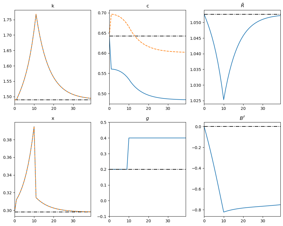
At time 1, the government announces that domestic government purchases
To smooth consumption, domestic households immediately increase saving, offsetting the anticipated hit to their future wealth.
In a closed economy, they would save solely by accumulating extra domestic capital; with open capital markets, they can also lend to foreigners.
Once the capital flow opens up at time
Because no-arbitrage equalizes the ratio of marginal utilities, the resulting paths of consumption and capital are synchronized across the two economies.
Up to the date the higher
When government spending finally rises 10 periods later, domestic households begin to draw down part of that capital to cushion consumption.
Again by no-arbitrage conditions, when
The domestic economy, in turn, starts running current-account deficits partially to fund the increase in
This means that foreign households begin repaying part of their external debt by reducing their capital stock.
36.11.3.2. Experiment 2: A foreseen increase in
We now explore the impact of an increase in capital taxation in the domestic economy
Because the change is anticipated, households in both countries adjust immediately—even though the tax does not take effect until period
shocks_global = {
    'g': np.full(S+1, g_ss),
    'g_s': np.full(S+1, g_ss),
    'τ_c': np.zeros(S+1),
    'τ_k': np.concatenate((np.zeros(10), np.full(S-9, 0.2))),
    'τ_c_s': np.zeros(S+1),
    'τ_k_s': np.zeros(S+1),
}

k0_ss, c0_ss = compute_steady_state_global(model, g_ss)
k_star = k0_ss
Bf_star = Bf_ss(c0_ss, k_star, g_ss, model)

init_glob = np.tile([k0_ss, c0_ss, k0_ss, c0_ss], S+1)

sol_glob = root(
    lambda z: compute_residuals_global(z, model,
            shocks_global, S, k0_ss, k_star, Bf_star),
            init_glob, tol=1e-12)

k, c, k_s, c_s = sol_glob.x.reshape(S+1, 4).T

# plot
fig, axes = plot_global_results(k, k_s, c, c_s, shocks_global, model,
                                k0_ss, c0_ss, g_ss, S, shock='τ_k')
plt.tight_layout()
plt.show()
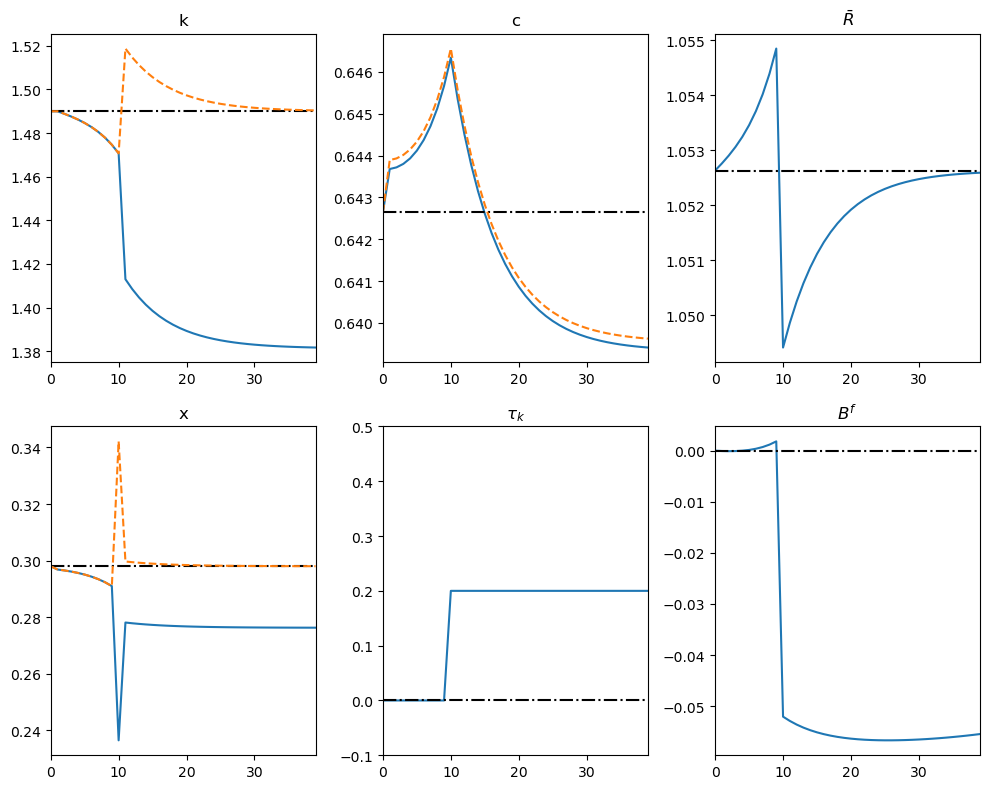
After the tax increase is announced, domestic households foresee lower after-tax returns on capital, so they shift toward higher present consumption and allow the domestic capital stock to decline.
This shrinkage of the world capital supply drives the global real interest rate upward, prompting foreign households to raise current consumption as well.
Prior to the actual tax hike, the domestic economy finances part of its consumption by importing capital, generating a current-account deficit.
When
The bond-rate drop reflects the lower after-tax return on domestic capital and the higher foreign capital stock, which depresses its marginal product.
Foreign households fund their capital purchases by borrowing abroad, creating a pronounced current-account deficit and a buildup of external debt.
After the policy change, both countries move smoothly toward a new steady state in which:
Consumption levels in each economy settle below their pre-announcement paths.
Capital stocks differ just enough to equalize after-tax returns across borders.
Despite carrying positive net liabilities, the foreign country enjoys higher steady-state consumption because its larger capital stock yields greater output.
The episode demonstrates how open capital markets transmit a domestic tax shock internationally: capital flows and interest-rate movements share the burden, smoothing consumption adjustments in both the taxed and untaxed economies over time.
Exercise 36.4
In this exercise, replace the plot for
Compare the figures for
Solution to Exercise 36.4
Here is one solution.
fig, axes = plot_global_results(k, k_s, c, c_s, shocks_global, model,
                                k0_ss, c0_ss, g_ss, S, shock='τ_k')

# Clear the plot for x_t
axes[1,0].cla()

# Plot η_t
axes[1,0].plot(compute_η_path(k, model)[:40])
axes[1,0].plot(compute_η_path(k_s, model)[:40], '--')
axes[1,0].plot(np.full(40, f_prime(k_s, model)[0]), 'k-.', lw=1.5)
axes[1,0].set_title(r'$\eta$')

plt.tight_layout()
plt.show()
When capital
This reflects that as capital becomes scarcer, its marginal product rises.